Volatility
For example, the sharpe ratio (excess returns / std deviation) while the utility function (Um = E(Rs,m) − 0.005 × λ × Variation)
Beta is a measure of a stock's volatility in relation to the overall market.
Risk is generally measured in terms of volatility, be it systematic (Beta via a regression) or idiosyncratic (std dev via a calculation).
Beta is a product of two factors: the relative volatility of the security's returns to the market's returns, and the correlation of the security's returns and the market's returns. Relative volatility is a part of it, but it is not solely a measure of volatility.
In other words, beta is correlated relative volatility or return-correlation adjusted relative volatility.
There are several ways to measure volatility, including beta coefficients, option pricing models, and standard deviations of returns.
Personally, in my portfolio I would like to have extremely low volatility of returns (with a positive mean) and extremely high volatility of prices.
Neither beta nor option pricing models is a measure of volatility. Beta is a measure of systematic risk, of which (relative) volatility is only a part. Option pricing models aren't measures of anything; the output of an option pricing model is an estimate of price (hence the name).
Measure the spread of returns around a mean
To annualize volatility, you multiply the periodic standard deviation by the square root of the number of periods in a year. This is because while returns are assumed to add up over time, their variance adds up linearly; therefore, the standard deviation (the square root of variance) must scale by the square root of time.
Daily Log Returns: Multiply by Sq 252 (252 trading days in a year).
Weekly Returns: Multiply by Sq 52
Monthly Returns: Multiply by Sq 12
24/7 Markets (e.g., Crypto): Multiply by Sq 365
Sharpe Ratio calculates risk-adjusted performance.
=(Ann_Ret - RF_Rate) / Ann_Vol
Sharpe Ratio Benchmarks:
< 1.0: Suboptimal.
1.0 – 2.0: Good.
2.0 – 3.0: Very Good.
3.0: Excellent.
daily log returns:
Compute the standard deviation of returns
If your dataset spans multiple years, you still annualize using the standard trading‑days convention:
Standard deviation is a common way to measure volatility. But it assumes a normal distribution of returns, which means it can struggle to account for real-world factors like skewness and kurtosis.
If this standard holds true, then approximately 68% of the expected outcomes should lie between ±1 standard deviations from the investment's expected return, 95% should lie between ±2 standard deviations, and 99.7% should lie between ±3 standard deviations.
In addition to skewness and kurtosis, a problem known as heteroskedasticity is also a cause for concern. Heteroskedasticity simply means that the variance of the sample investment performance data is not constant over time. As a result, standard deviation tends to fluctuate based on the length of the time period used to make the calculation, or the period of time selected to make the calculation.
Exploring the Historical Method for Volatility Analysis
Fortunately, there is a much easier and more accurate way to measure and examine risk, through a process known as the historical method. To utilize this method, investors simply need to graph the historical performance of their investments, by generating a chart known as a histogram.
A histogram is a chart that plots the proportion of observations that fall within a host of category ranges. For example, in the chart below, the three-year rolling annualized average performance of the S&P 500 Index for the period of June 1, 1979, through June 1, 2009, has been constructed. The vertical axis represents the magnitude of the performance of the S&P 500 Index, and the horizontal axis represents the frequency in which the S&P 500 Index experienced such performance.
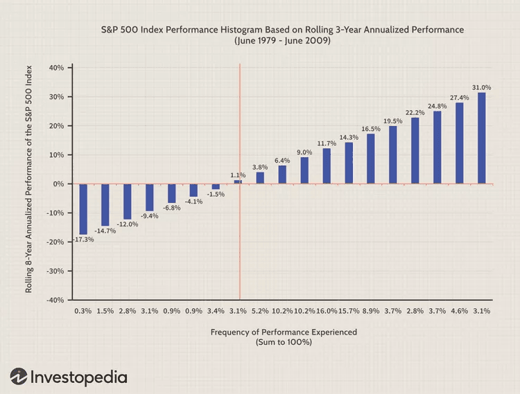
As the chart illustrates, the use of a histogram allows investors to determine the percent of the time in which the performance of an investment is within, above, or below a given range. For example, 16% of the S&P 500 Index performance observations achieved a return between 9% and 11.7%. In terms of performance below or above a threshold, it can also be determined that the S&P 500 Index experienced a loss greater than or equal to 1.1%, 16% of the time, and performance above 24.8%, 7.7% of the time.
