Non-ergodicity
The following conundrum is like one that Peters used but illustrates the point a little better.
Suppose a casino makes the following offer. You bet a sum of money and the casino tosses a fair coin. If the coin comes up heads the casino will give you a 50% return on your bet; that is, you win five dollars for every 10 dollars that you bet. If the coin comes up tails you lose 40%; that is, for every 10 dollars you bet you walk away with only six dollars.
This is stupid of the casino, because for every four dollars it gains it gives away five dollars. To put it in Peters’ terms, its “ensemble average” return on your bet is negative. It is minus 5% (the average of -50% and +40%). “Ensemble average” is the same thing as “expected return” in probability language. It’s a clear loser for the casino.
But it’s also a loser for the gambler. On average over time, for every +50% return the gambler gets because a head was tossed, the gambler will see a tail tossed and get a -40% return, because as the sequence of tosses grows longer, the ratio of heads to tails approaches one. And although +50% and -40% average to +5%, they compound to a 10% loss (1.5x0.6=0.9).
You might have thought the gambler would win over time since her ensemble return (expected return) is plus 5%, but that’s not the case. That is because the time-average return does not equal the ensemble return – this is technically called “non-ergodicity.”
Here, for example, is a randomly-generated sequence of the results of 40 coin tosses (H for heads, T for tails):
TTTTHTHHHHHTHTHHTTTTHTHHHTHHHHHTTHHHTTTT
There are 21 heads and 19 tails, so the bettor wins 21 times and loses 19 times. If the bettor initially bets 10 dollars and lets it ride, she will end up with $10 x 1.521 x 0.619 or about three dollars, less than a third of what she started with.
How can this possibly be? Gambling against a casino is a zero-sum game. It’s not possible that both the gambler and the casino lose.
What is the solution to this conundrum?
The solution
The gamblers do not lose in their 40-toss “ensemble average” – in fact they win. If you average the gains and losses of many gamblers in the casino betting on 40 tosses it will turn out that on average, their initial $10 bet comes to $70.
That’s weird, you may say, any one gambler loses big over time, but on average they win big? How is this possible?
It happens because the distribution of 40-coin gains and losses is fat-tailed. To a close approximation it’s a highly skewed lognormal distribution. Most people lose, but a few win so big that it skews the average far to the positive.
Only a lucky few winners on the distribution’s tail take advantage of the stupid casino. The rest are losers.
This interesting insight powers much of Peters’ work. (Remember this example – we’ll revisit it later.)
But should I take the bet?
Straining for a practical implication
You may ask, so what? Does this have any practical application – for example, to investment management?
The answer is no, not really – or at least, not yet.
Nevertheless, not only Peters but also institutional investment consulting firms that have been enthralled by Peters’ tantalizing insights imply that it does have important practical implications – without quite specifying what.
For example, this post by the consulting firm Willis Towers Watson presents an extended version of Peters’ conundrum. Then, although it contains a section on practical implications, it doesn’t explore it in any detail.
I will do that.
I will explore an important and – according to Peters – practical implication, in detail.
Peters’ claim of an application to portfolio optimization
Peters’ argument for what is wrong with the current theory and practice in economics, and what should be done instead proceeds in three claims:
- Optimizing the expected value of wealth (or “ensemble average”) is flawed because for non-ergodic processes (such as investment returns over time), the time average doesn’t equal the ensemble average.
- In economics this flaw is patched up by maximizing not expected wealth, but the expected “utility” of wealth. However, says Peters, this is also flawed because instead of making an objective judgment of optimality it jumps to “psychological arguments,” thus “appealing to subjective psychology” or “other forms of personalization.”
- The solution is to convert the wealth growth process to an ergodic process by maximizing the expectation of the logarithm of wealth instead of either wealth itself or the utility of wealth.ii This is equivalent to the well-known Kelly criterion, which was proposed in 1956 by John Kelly, a researcher at Bell Labs.
In a 2011 paper that was published in the journal Quantitative Finance titled “Optimal leverage from non-ergodicity,” Peters discussed the solution proposed by #3 in the context of the portfolio optimization problem. However, that paper doesn’t give any examples of the application of that solution.
I will provide one.
I’ll look at its application to optimizing a portfolio’s stock-bond mix. I’ll use the following assumptions: expected return and standard deviation of stock returns, 7% and 18%, respectively; expected return and standard deviation of bond returns, 2% and 7%, respectively; and I will assume zero correlation between them.
The result of maximizing the expectation of the logarithm of return is a highly leveraged portfolio. The optimum calls for 193% stocks. To implement this, the investor would have to borrow 93% of her invested wealth to invest 193% of it in stocks.
But this result is very sensitive to assumptions. Table 1 shows optimal allocations for various assumptions.
Table 1. Optimization of stock-bond mix by maximizing expected logarithm of return, for various equity return and standard deviation assumptions

Is the 193% equity solution good? Perhaps a leveraged hedge fund would be interested in implementing it. But maximizing the expected value of the logarithm of return wouldn’t give it much guidance, because the result is entirely dependent on the equity and bond return assumptions used as input. Garbage in, garbage out.
Peters’ claim of an application to insurance
In a well-written 2017 paper titled, “Insurance makes wealth grow faster,” Peters and co-author Alexander Adamou attempted to show another application of solution #3, this time to insurance. They first argued that if they used the flawed approaches defined by points #1 and #2 above, either nobody would want to buy insurance, or no insurer would be willing to provide it, because it would always appear to be a loser for one or the other.
But by using solution #3 – maximizing the expected logarithm of wealth – and choosing their assumptions very carefully, Peters and Adamou present a case in which the same contract is optimal for both the insurer and the insured.
The trouble with this is that the insurer and the insured have different objectives. In my casino example above, the gambler’s objective may be to get the best result over time, but the casino’s objective is – or should be – to maximize its ensemble average.
This crucial distinction is even made by Nassim Taleb himself in an invaluable book that he sent me – and that I will mention again later – titled, “Statistical Consequences of Fat Tails.” There he says, “we can compute the casino’s return using the law of large numbers by taking the [average] return of the 100 people who gambled… The problem comes when ensemble probability is applied to us as individuals.”
The same is true of insurance. The insurer doesn’t have the same optimization objective as the insured. And that is why insurance works, not because both the insured and the insurer maximize the expected logarithm of their wealth. The insurance company earns a profit precisely by intermediating between the over-time concern of its customers and its own financial concern, namely its ensemble average.
Does personal wealth grow randomly?
In three other papers, on a different subject, Peters and Adamou are onto something. They should explore it further. (Two of the papers are also co-authored with Yonatan Berman.)iii
In those papers they assume that personal wealth grows according to geometric Brownian motion. They’re not talking here only about an individual’s investment wealth, which is usually assumed in technical papers to grow according to geometric Brownian motion. They’re talking about all the individual’s wealth.
They make this assumption in their mathematics, but curiously don’t talk about the extensive implications of that assumption.
The implication of assuming geometric Brownian motion for an individual’s investments is either the efficient market model or another theoretical explanationiv. It assumes that invested assets grow randomly, because future investment returns are independent of past investment returns.
But does an individual’s entire wealth grow randomly? This is counterintuitive.
We assume that some individuals are not merely lucky, but more skilled at growing their wealth than others – not because they’re better at forecasting the stock market, but because they have other wealth-building advantages, for example better education, higher intelligence or more advantageous parentage.
However, though Peters, et al., don’t explicitly tease out this theme, they do argue – and show – that inequalities in wealth can be adequately explained entirely by this random wealth-growth hypothesis, even the high levels of wealth inequality that we’re seeing now.
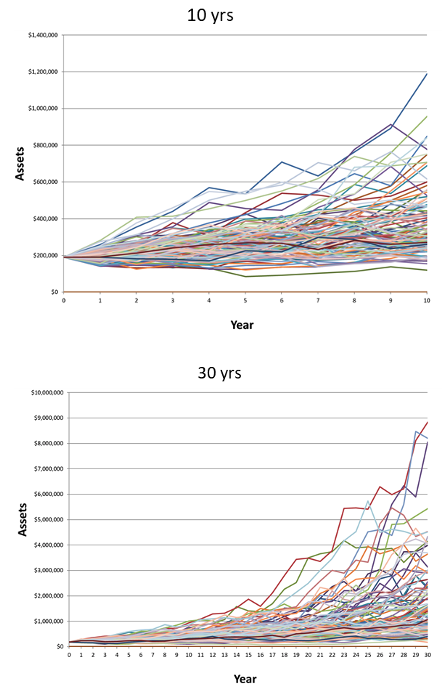
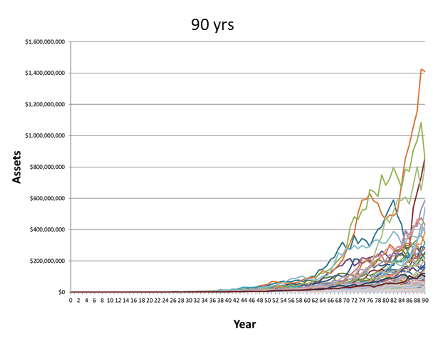
Figure 1, which I have generated using Monte Carlo simulation, shows how much wealth inequality increases over time merely by virtue of random wealth growth. Note the enormous increase in inequality, from 10 years of random wealth growth to 90 years. The upper tail of the distribution grows farther and farther away from the cluster at the bottom.
Figure 1. Random growth of wealth over 10, 30, and 90 years
Peters, et al., then had the ingenious idea to model wealth growth using what I will call “punctuated geometric Brownian motion.” Periodically, the geometric Brownian motion process of wealth growth is modified by a redistribution of wealth, perhaps through government action or some other cause. They call this model “reallocating geometric Brownian motion,” or RGBM.
They fit this model to wealth growth data obtained from a prominent paper by E. Saez and G. Zucman titled, “Wealth inequality in the United States since 1913: Evidence from capitalized income tax data.” One might assume that redistributions of wealth go from the wealthier to the less wealthy, but Peters and his coauthors found this not to be the case in recent years – in fact according to their model (whose assumptions may be highly debatable and must of course be kept in mind), in recent years the reallocation as compared with mere randomness of growth has been from the less wealthy to the wealthiest.
The relationship to Taleb’s project
Let’s go back to the casino example and its offer of a coin toss. In a 40-toss sequence most bettors lose – in fact 78.52% of them – but on average they win $60. Their average final wealth, combined with their initial $10 bet, comes to $70.
The exact figure is $69.67, a number that can be calculated from probability theory.
However, that number can also be estimated “empirically” – or quasi-empirically – by generating many sequences of 40 random coin tosses and averaging the winnings. If you generate 10 million such sequences and average their final wealth you get very close to the correct figure of $69.67.
But if you “only” generate 10,000 sequences and average them, then your estimate of the average ending wealth may not get close at all. Generating 10 averages of 10,000 sequences typically yields estimates of average ending wealth ranging from $50 to $106. And if you generate only 500 sequences the estimates of average ending wealth range from $21 to $237.
How can these estimates of the average vary so widely when there are 500 samples that are all drawn perfectly randomly from the population they represent?
It’s because of the strongly skewed lognormal distribution of final wealth, which renders the estimate of its average seriously unreliable. > From <https://www.advisorperspectives.com/articles/2021/03/01/understanding-fat-tail-returns?topic=insurance-annuities>
